New Panorama Cameras

I made two cool new cameras that allow the entire sky to be viewed in a single image.

The first uses latitude-longitude panoramic format, also known as an equirectangular mapping. This is the same format that I use for HDR environment maps in Photorealizer, and my sky renderer already saves images to EXR (in addition to PNG), so I will be able to use my sky renderer renders as HDR environment maps for my Photorealizer renders. Plus, I have HDR environment map importance sampling in Photorealizer, so I can leave the tiny, bright, influential sun in the sky images and Photorealizer will automatically know to heavily sample the sun.

Equirectangular projection.

The second new camera uses an angular fisheye projection. This is a pretty intuitive way to view the entire sky (and part of the ground in my implementation). This kind of picture can be captured in real life in a single shot with a fisheye lens. Real fisheye lenses are pretty advanced. Here is a site that shows how a real fisheye lens works, with nice diagrams of the fancy optics.

Angular fisheye projection.

The environment is identical in both images above. The solar elevation angle is 10°. I think that the two bright peaks above the horizon in the solar and anti-solar directions are due to the forward and backward peaks of the Rayleigh scattering phase function.

Vertical Distribution of Ozone

I noticed that the sky right above the horizon seemed too blue after I implemented ozone absorption. I realized that since the most Rayleigh scattering happens in the low, dense part of the atmosphere near the ground, scattered light would be passing through too much ozone if the concentration were too high at these altitudes. I also thought more generally about the geometry of the atmosphere and the differing amounts of ozone that light would pass through based on the distribution of the ozone. I had made the ozone concentration a constant value of 0.6 parts per million, which had made the total ozone amount correct, but it had also made the amount near the ground far too high, and the amount higher in the atmosphere far too low. That amount of ozone at ground level would be dangerous to your health. In reality, most of the ozone in the atmosphere is found in the ozone layer in the stratosphere. The ozone layer is responsible for absorbing most of the sun's harmful UV rays.

To improve my results, I implemented a realistic distribution of ozone. Average data for the Earth's atmosphere was difficult to find, and the exact distribution of ozone is pretty variable anyway, so I read data from the NASA graph below, and made a few tweaks based on other information I had found (namely, lowering the concentration in the troposphere, and weighting the data up to make the total concentration closer to 0.6 ppm). I might want to tweak or replace the data in the future, but it's already much more accurate than the constant value I was using before.

Ozone concentration in the atmosphere. Image from NASA.

Below is a new render, and some old ones for comparison. In the new render, compared to the old ozone render, the sky around the zenith is bluer, and the the color and brightness near the horizon is more accurate.

Ozone with realistic vertical concentration profile.

Ozone with uniform concentration throughout the atmosphere.

No ozone.

Here's another new render, this one taken during twilight in the direction of the sun, with the sun −3° below the horizon:

Twilight + ozone.

By the way, ozone absorption should make the color of the Earth shadow at twilight more accurate (darker and bluer), so I'm looking forward to rendering some shots that illustrate that.

Ozone Absorption

A couple weeks ago, I noticed that, in my sunset and twilight renders, towards the zenith, the sky looked fairly gray, while in real life it looks fairly blue. I realized that implementing the actual solar spectral irradiance would make the sky appear slightly bluer, but I didn't expect the effect to be strong enough to explain the discrepancy between my images and real life. Then I stumbled across something very interesting on Wikipedia:

According to Craig Bohren, "preferential absorption of sunlight by ozone over long horizon paths gives the zenith sky its blueness when the sun is near the horizon".

I proceeded to check the referenced Craig Bohren paper, where the statement was explained in more detail. In particular, the Chappuis absorption band of ozone, "which extends from about 450 to 750 nm and peaks at around 600 nm", is responsible for absorbing light of longer wavelengths in the visible spectrum, thus making the sky appear more blue. He also said that

In the absence of molecular absorption, the spectrum of the zenith sky would be essentially that of the zenith sun (although greatly reduced in radiance)

Bohren referenced a 1953 paper by Hulbert, who originally pointed out this explanation of this blueness: Explanation of the Brightness and Color of the Sky, Particularly the Twilight Sky. Here's an excerpt from the abstract of that paper:

Calculation showed that during the day the clear sky is blue according to Rayleigh, and that ozone has little effect on the color of the daylight sky. But near sunset and throughout twilight ozone affects the sky color profoundly. For example, in the absence of ozone the zenith sky would be a grayish green-blue at sunset becoming yellowish in twilight, but with ozone the zenith sky is blue at sunset and throughout twilight (as is observed), the blue at sunset being due about 1/3 to Rayleigh and 2/3 to ozone, and during twilight wholly to ozone.

I also found a paper from 1973, The Influence of Ozone and Aerosols on the Brightness and Color of the Twilight Sky, that confirms the effect of ozone on the color of the twilight sky using computer simulations.

I decided that I needed to include ozone absorption in my sky renderer, so I searched around for spectral ozone absorption data, and eventually came across recent (2011), high-precision, absorption cross-section measurements here. The data is provided in 0.01 nanometer increments, which is way too precise for my purposes, so I wrote some code to convert the data to 5 nanometer increments, averaging 500 data points to create each new data point. The data is provided for 11 different temperatures. They're similar enough that I probably could have just used one, or averaged them all together, but I decided to use all of them anyway. When a query is made, I just look up the data at the closest temperature and wavelength—I decided that interpolation was probably overkill in this case.

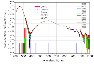
Ozone absorption cross-sections. Image from IUP.

To convert the absorption cross-sections (units of cm^2/molecule) to absorption coefficients (units of cm^-1), I multiply by the molecular number density of standard air (units of molecules/cm^3), multiply by the concentration of ozone in the atmosphere (unitless), and then correct for altitude by multiplying by the relative density (unitless) at the altitude in question. The concentration of ozone varies a lot with altitude, but I just used the overall concentration, which is around 0.00006% (I wonder to what extent a more realistic distribution would affect my results). I packaged all of this up in a new Ozone class.

Below are some new renders with and without ozone absorption. These images are taken during twilight, looking straight up along the zenith.

Twilight zenith sky with ozone.
Solar elevation angle: −5°.

Twilight zenith sky without ozone.
Solar elevation angle: −5°.

Below are some more new renders (all with the same exposure) that show the effect of ozone absorption on the color of the sky. The previously intense orange at sunset is now much more subdued. The orange should become somewhat more saturated when I add aerosols to the atmosphere—an effect described in The Influence of Ozone and Aerosols on the Brightness and Color of the Twilight Sky and in Color and Light in Nature.

With ozone.
Solar elevation angle: 1°.

Without ozone.
Solar elevation angle: 1°.

With ozone.
Solar elevation angle: 30°.

Without ozone.
Solar elevation angle: 30°.

I'm pretty excited about these results. I think it's very interesting that Rayleigh scattering alone does not explain the blueness of the sky. According to The Effect of Stratospheric Dust on the Color of the Twilight Sky, adding dust will increase the blueness of the twilight sky even more. I wonder whether implementing absorption by other gases would have any other noticeable effects on my results.

By the way, as far as I know, the existing sky simulations and analytic sky models in computer graphics do not consider the effects of ozone absorption.

Spectral Solar Irradiance

Image created by Robert A. Rohde / Global Warming Art

I implemented the spectral irradiance of the sun based on modern AM0 data. AM0 (Air Mass Zero) means that the data is for sunlight that hasn't passed through any atmosphere, which is what I needed because I am simulating the atmosphere myself. This extraterrestrial spectral solar irradiance data is often used for space applications. AM1.5 data is also available, for ground level applications such as solar energy. I found the data on NREL's website, and it originally came from a 2003 paper by Guemard. In my renderer I convert irradiance to radiance instead of using the data directly. Previously, I was using a constant value for the sun's energy, uniform across the spectrum. I could have alternatively used a black body radiation curve to approximate the spectral irradiance, however spectral solar irradiance does not exactly follow a black body radiation curve.

Here are some renders comparing the new and old solar spectra. To clearly see the differences, you can click an image to bring it up in the lightbox, then you can then switch between images. One of the most noticeable differences is that the new images are bluer.

New.

Old.

New.

Old.

To use the spectral solar irradiance data, I wrote a LookupTable class with a custom binary search and linear interpolation, and then made a SpectralSolarIrradiance subclass with an array of wavelength keys and spectral irradiance values. I made another subclass of LookupTable called RayleighScatteringDepolarizationFactor to store the depolarization factor data for Rayleigh scattering. I could also make my CIEXYZColorMatchingFunctions class extend the LookupTable superclass, however it currently uses optimized code that I wrote specifically for data given in uniform increments. I will probably also use the LookupTable class for ozone absorption data. Ozone absorption is an important factor that I will write about in a future post. I also now have new classes for USStandardAtmosphere1976, RayleighScattering, which I didn't write right away just because the code was in a lot of flux. I'll post more information about the structure of my code another time.

Shadow of the Earth

When flying from San Francisco to Los Angeles this summer, we took off right before sunset, and I was lucky enough to have a window seat. As we emerged from the clouds into the clear sky above, I had a brief but amazing view of the bright orange sun shining and scattering through the clouds. I was on the left side of the plane, so as we turned to the south, the view of the sun went away, but the sun set soon anyway.

What I saw after the sun had set was really remarkable. The sky was very clear, and above the horizon I started noticing an expansive dark area with a pretty sharp edge, gradually consuming the sky. I soon realized that what I was seeing was the shadow of the Earth in the atmosphere. Inside the shadow, the sun had already set, but in the brighter area above the shadow, the sun would have still been directly visible.

I am able to replicate this effect in my sky renderer.

Here's a render at twilight, from the ground, facing away from the sun. You can clearly see the shadow of the Earth in the lower part of the image above the horizon (the ground is the sharp, rectangular, solid-colored area at the bottom). You can even see the anti-twilight arch!

Twilight, facing
away from sun.

And below is my earlier twilight render, looking in the direction of the sun, for comparison. The exposure on this image is three stops lower than the shadow image above. I raised the exposure on the image above because the sky was much darker in the direction opposite the sun.

Twilight, facing
towards sun.

Visible Spectrum

Here's what the visible spectrum looks like at a few different exposures when rendered in my sky renderer. I used my new spectral rendering and display system (spectrum → CIE XYZ → linear RGB → sRGB) to create these images.

CIE XYZ

The sRGB gamut in the CIE xy chromaticity diagram.
Image found on Dietrich Zawischa's colorimetry page.

One of the first things I did for this project is to write a spectral rendering system that associates each ray with a wavelength instead of an RGB color. Initially, in order to convert the spectral data to RGB primaries, I made up response curves for the camera's RGB sensors, but this was just a rough placeholder system. I considered implementing the response curves of a real-life camera, however, I decided on a more scientific approach. I decided to convert my spectral data to CIE XYZ by integrating it with the CIE XYZ color matching functions (specifically, the CIE 1931 2° XYZ CMFs modified by Judd and Vos), then transforming XYZ to linear RGB (Rec. 709 primaries), then finally transforming that to sRGB. This approach yields colorimetrically accurate results and is very flexible. I'm very interested in color, so doing this was also fun and good practice.

Here are after and before shots of twilight. Notice how the hues shift:

Updated twilight
image.

Old twilight image,
for comparison.

Here are a few more new renders:

Updated day
image.

Notice the multicolored noise in this quick render, resulting from spectral rendering coupled with Monte Carlo scattering:

Updated sunrise /
sunset image.

Latest Results

Below are some renders I made after implementing direct sun sampling. these are images of a clear, dry sky, with only Rayleigh scattering and no Mie scattering.

I have not yet implemented a realistic spectral emission distribution for the sun, so right now, it's just flat across the visible spectrum. I am using a rough, temporary approach to convert spectral results to RGB. These pictures all use the same exposure, so the luminosities are roughly comparable.

For now, I made the ground an 18% gray, perfectly diffuse reflector.

Sunrise or sunset.

Twilight. Sun
below horizon.

Day.

Day with
lower sun.

Sampling the Sun Directly

The sun covers only a tiny fraction of the sky, about 0.00047%, so with naive path tracing, most rays would get lost in space and the image would take forever to converge. By sampling the Sun directly, I was able to speed up my simulation tremendously. At each scattering point, I fire a ray directly towards the Sun, weighted by the Rayleigh scattering phase function in that direction, and weighted by the probability that a ray fired in a random direction would hit the sun. I also still fire a scattered ray in a direction drawn from the Rayleigh scattering phase function, however this ray cannot "see" the Sun. If I were to only sample the Sun, I would lose multiple scattering, which plays an important role in the appearance of the sky. For computing sample directions that are uniformly distributed over the solid angle subtended by the Sun (the Sun is not a point light or a directional light), I used the Sun class that I wrote for Photorealizer.

Ray Marching

Because the properties of the atmosphere vary with altitude, I can't just use the scattering and absorption properties at a single point to compute scattering and absorption along a ray. Instead, I implemented a ray-marching system that takes fixed-size steps along each ray. Each step forms a line segment. For each segment, I use the altitude, density, and Rayleigh scattering coefficient from the midpoint of the segment, and assume that these properties are constant along the span of the segment. This allows me to compute a random scattering distance (or absorption distance, but I've only implemented Rayleigh scattering so far) by importance sampling the exponential falloff of unscattered light. If the sampled scattering distance is less than the length of the segment (i.e., if the scattering point falls within the segment), I scatter it, otherwise I proceed to the next segment. By decreasing the step size, the simulation can be made more accurate, but you get diminishing returns at a certain point, slowing down the program without a noticeable increase in accuracy. I am considering implementing adaptive step sizes based on the density of the air.