Comparison

Here's a current render from my sky simulator compared with one from Hosek and Wilkie's (one of the path tracer renders from their paper, scaled up to the same size as my render). I purposely matched the lens, the solar elevation angle, and the exposure, however I did not try to match the atmospheric properties, ground albedo, or tone-mapping. There are a few images in the Hosek–Wilkie paper with a solar elevation angle of 4°, and I simply chose the one that matched my render from the previous post most closely (which was the one with a turbidity of 6), then I re-exposed my (HDR) render to match the Hosek–Wilkie one as well as possible. Besides the numerous differences in the simulations themselves, there a few notable differences between these two images: Hosek and Wilkie's is tone-mapped while mine is not, mine uses a fisheye lens that extends beyond 180° to show the ground, and mine includes the solar disc. In spite of the differences, the images look remarkably similar to me. Using the lightbox, you can toggle between the two images.

My sky simulator.

Hosek and Wilkie's sky simulator.

Aerosols

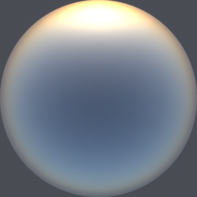
With aerosols. Solar elevation angle 4°.

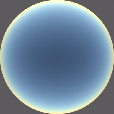
No aerosols. Solar elevation angle 4°. Same exposure as the image above.

I made a first pass at adding aerosols to the atmosphere. Aerosols have a significant impact on the appearance of the sky, but simulating them isn't particularly straightforward: the types and levels of aerosols vary widely by region (e.g., city vs. forest vs. ocean) and other factors, and computing their scattering properties is quite complicated.

I used the representative profile of aerosols in Elterman's paper UV, Visible, and IR Attenuation for Altitudes to 50 km, 1968. The paper provides aerosol extinction coefficients that vary based on altitude and wavelength. It's the same data used in The Influence of Ozone and Aerosols on the Brightness and Color of the Twilight Sky, which is what led me to the paper in the first place. I used the provided scale height relationship (scale height of 1.2 km) to extrapolate the data beyond 50 km.

For the scattering phase function, for now I just used the Henyey-Greenstein phase function, which I had already implemented for Photorealizer, including analytic scattering direction sampling. For now I used a constant asymmetric parameter of 0.7 (which means that the mean cosine of the scattering angle is 0.7, which implies strong forward scattering), which seems to be a pretty good average value based on my research. I plan to implement Cornette and Shanks's modified version of the Henyey-Greenstein phase function, which better approximates actual Mie scattering phase functions and converges to the Rayleigh phase function as the asymmetry parameter approaches zero.

I used a constant single scattering albedo of 0.9, which, like my asymmetry parameter, seems to be a pretty good average value based on my research. At the sampled extinction distance, I scatter the photon/ray with 90% probability, and absorb it with 10% probability.

I changed the Earth's surface to have an albedo of 31%, which seems to be the accepted average albedo of Earth's surface. At some point, I would like to make a procedural ground, or use a map of the actual Earth. Procedural mountains would be particularly nice for showing off atmospheric effects.

My aerosols system could be improved in many ways. In particular, I could use a realistic particle size distribution, use realistic particle type proportions (each type having a certain index of refraction, with real and imaginary parts), and then compute scattering and absorption properties using the Mie solution to Maxwell's equations. That sounds like it might be overkill for now, although I'm sure I would learn a lot in the process. 

Unbiased Distance Sampling

I implemented an algorithm for unbiased distance sampling in heterogeneous media, which replaces the biased ray marching in my sky renderer. It's a Monte Carlo algorithm, "Algorithm 1" in the paper Unbiased Global Illumination with Participating Media. I learned about that paper from Hosek and Wilkie's sky model paper. The algorithm originates from a 1968 paper by Coleman, which I'm interested in looking at, but which I haven't been able to locate.

The algorithm samples a random distance based on the highest extinction (or scattering or absorption) coefficient along the ray (or line segment in my case), or any coefficient greater than or equal to that (such as the highest in the entire medium, which is often easier to find). Then it probabilistically takes another leap based on the actual coefficient at the sampled location.

Algorithm from Unbiased Global Illumination with Participating Media.

Using the lowest max coefficient allows larger steps to be taken, which decreases the number of steps needed and increases performance. Since Rayleigh and ozone scattering and absorption coefficients vary predictably based on wavelength, the lowest max coefficient can be found for given wavelength, and with Rayleigh scattering, the lowest coefficient along the line segment can be found by using the coefficient at the point on the line segment that is closest to the center of the Earth (assuming density is monotonically decreasing with altitude).

After implementing this algorithm and the related optimizations, not only are my renders unbiased, but they are also 5 to 10 times faster—a pretty huge speed increase.

Earth from Space

Because I'm performing a brute force atmospheric simulation, I'm able to render the atmosphere from any point of view. After a few tweaks, I'm now able to render images from outside the atmosphere. Here are a few images that show what the Earth looks like from space. The planet's surface is currently an 18% gray Lambertian diffuse reflector.

The planet as seen from 200 km up.

Same view as above, but with no atmosphere.

A different view. Also 200 km up. Sun right below the horizon.

Adaptive Step Size

To increase accuracy and significantly decrease simulation times, I made the ray marching step size vary based on a few heuristics: the rate of change of the altitude at the current location, the altitude of the current location, and an element of randomness.

The first heuristic, the rate of change of the altitude, has the biggest impact on the step size. When a short line segment is nearly parallel to the ground, the altitude doesn't varying much along the segment, which means that the density and other properties of the air also don't vary much along the segment. So if we're travelling parallel to the ground we can take much larger step sizes than if we're travelling perpendicular to the ground. When we're travelling up and down, the atmospheric properties change much more quickly and we need to smaller step sizes to accurately capture the changes and details of atmospheric properties.

These are all just a temporary improvements because I just realized that I could replace ray marching with an unbiased technique, which should also be cleaner and faster. I'll write more about this later, after I implement it.

If I were to stick with ray marching, I would want to additionally vary the step sizes based on wavelength and other factors, and I would want to take different step sizes when computing different types of scattering and absorption.

Twilight Fisheye

Here's a new angular fisheye render taken at twilight (solar elevation angle −3°) in which you can clearly see the twilight arch, the anti-twilight arch, and the Earth shadow.

To produce the image below, I first took advantage of the symmetry of the render to effectively double the number of samples, using Photoshop to duplicate the high-dynamic range EXR image, flip it horizontally, and composite it onto the original. Then I used Photomatix to tone-map the processed image. The solar (top) side is much brighter than the anti-solar (bottom) side, so without tone-mapping it wouldn't be possible to expose the entire sky nicely at one time—part of the image would be overexposed or part would be underexposed. The tone-mapped image is over-saturated and the relative intensities of different parts of the sky are not accurate, but you can see the entire sky and you can see the colors clearly.

Twilight, tone-mapped.

And below is the PNG that came directly out of my renderer. I applied a mild S-shaped transfer curve before writing to PNG.

Twilight, directly from my renderer.

The sky was clear this evening in Philadelphia and I was able to see the Earth shadow. The colors in the real sky closely resembled those in this render.